This post briefly sketches out the types of bootstrapped confidence intervals commonly used, along with code in R for how to calculate them from scratch. Specifically, I focus on nonparametric confidence intervals. The post is structured around the list of bootstrap confidence interval methods provided by Canty et al. (1996). This is just a quick introduction into the world of bootstrapping - for an excellent R package for doing all sorts of bootstrapping, see the boot package by Brian Ripley.
Suppose that $x_1, x_2, …, x_n \sim f(\theta)$, where $f(\cdot)$ is some arbitrary probability distribution. We are interested in estimating $\theta$. Let $\hat{\theta}$ be the point estimate of the parameter of interest obtained from the original dataset. Note that these are nonparameteric confidence intervals (that is, we don’t assume that $f$ is a particular parametric family). The example comes from page 201 of DiCiccio and Efron (1996), which contains a dataset on five exams across 22 students (with some missing data). The parameter of interest is the maximum eigenvalue of the empirical covariance matrix. You may download the data here. The code for estimating the max eigenvalue is provided at the end of this post. The function is called calculate.max.eigen.
Using this function on the dataset, we obtain $\hat{\theta}=216.2$.
Now, suppose that we bootstrap the dataset M times and for each of the datasets, calculate $\hat{\theta}^*_{m}$, which is the point estimate of $\theta$ for the mth bootstrapped dataset. The empirical distribution of $\hat{\theta}^*$ is the bootstrap distribution and is an approximation to the sampling distribution for $\hat{\theta}$.
To create $M=10000$ bootstrap replicates in R:
BS.eigen <- function(data){
    index <- sample(1:nrow(data),size=nrow(data),replace=TRUE)
    bs.data <- data[index,]
    return(calculate.max.eigen(bs.data))
}
bs.sampling <- replicate(10000,BS.eigen(data),simplify=TRUE)
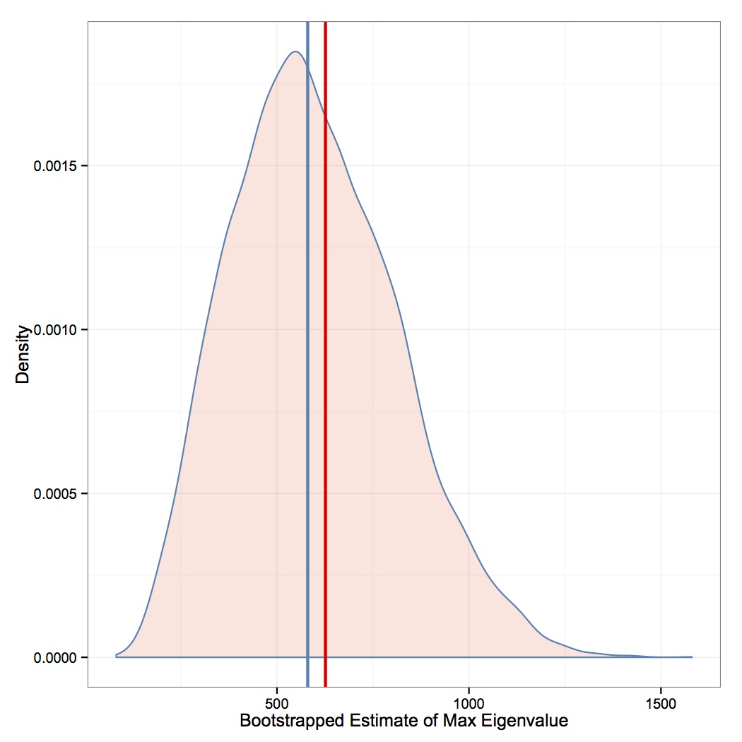
Here is the distribution of these estimates (with the median of the bootstrapped estimates denoted with the vertical blue line and $\hat{\theta}$ denoted with a vertical red line):
We can then make use of the bootstrap distribution in a number of ways to obtained bootstrapped confidence intervals.
Normal intervals
\(\hat{\theta} \pm z_{\alpha/2} \sigma_{bs},\) where $z_{\alpha/2}$ is the $\alpha/2$-quantile of the standard normal distribution and $\sigma_{bs}$ is the standard deviation of the bootstrap distribution. These intervals are justified by asymptotic theory (Central Limit Theorem).
In R:
theta.hat + qnorm(0.025)*sd(bs.sampling)
theta.hat + qnorm(0.975)*sd(bs.sampling)
For our example, we obtain a confidence interval of [202.64,1050.01].
Transformed normal intervals
\(t^{-1}[t(\hat{\theta}) \pm z_{\alpha/2} \sigma_{tbs}],\) where $t(\cdot)$ is a variance-stabilizing square root transformation and $\sigma_{tbs}$ is the standard deviation of the transformed bootstrap distribution (distribution of $\hat{\theta}^*$).
In R:
(sqrt(theta.hat) + qnorm(0.025)*sd(sqrt(bs.sampling)))^2
(sqrt(theta.hat) + qnorm(0.975)*sd(sqrt(bs.sampling)))^2
For our example, we obtain a confidence interval of [263.67, 1143.33].
Basic bootstrap intervals
\[[2\hat{\theta}-\hat{\theta}^*_{m=(1-\alpha/2)M}, 2\hat{\theta}-\hat{\theta}^*_{m=(\alpha/2)M}]\]
In R:
2*theta.hat - quantile(bs.sampling,0.975)
2*theta.hat - quantile(bs.sampling,0.025)
For our example, we obtain a confidence interval of [186.45, 1018.62].
Transformed basic bootstrap intervals
These are basic bootstrap intervals with similar transformation to the transformed normal intervals.
In R:
(2*sqrt(theta.hat) - quantile(sqrt(bs.sampling),0.975))^2
(2*sqrt(theta.hat) - quantile(sqrt(bs.sampling),0.025))^2
For our example, we obtain a confidence interval of [302.76, 1208.00].
Percentile confidence intervals
\[[\hat{\theta}^*_{m=(1-\alpha/2)M},\hat{\theta}^*_{m=(\alpha/2)M}]\]
In R:
quantile(bs.sampling,0.975)
quantile(bs.sampling,0.025)
For our example, we obtain a confidence interval of [233.93, 1066.10].
BCa confidence intervals
A refinement on the percentile confidence interval method, designed to increase accuracy. Note that BCa reduces to standard percentile confidence intervals if the bootstrap distribution is unbiased (median of the distribution is equal to the original point estimate) and the acceleration (skewness) is zero.
Step 1: Calculate the bias-correction $\hat{z}_0$, which gives the standard normal quantile function of the proportion of bootstrapped estimates less than the original point estimate: \(\hat{z}\_0 = \Phi^{-1} \left\[\dfrac{\sum \{\hat{\theta}^\* < \hat{\theta} \}}{M} \right\]\)
In R:
z0 <- qnorm(mean(bs.sampling < theta.hat))For our example, $\hat{z}_0$ is 0.194, which indicates a positive bias correction. This follows from the fact that 57.7% of $\hat{\theta}^*$s are below the original point estimate $\hat{\theta}$ (downward bias). We can see this from the plot above since the median of the bootstrap distribution is to the left of the point estimate from the original dataset.
Step 2: Calculate the acceleration $a$, which has an interpretation of skewness (more specifically, it measures how rapidly standard error changes on a normalized scale). A non-parametric estimate of $a$ is: \(\hat{a} = \dfrac{1}{6}\dfrac{\sum_{i=1}^n (\hat{\theta}-\hat{\theta}_{(i)})^3}{(\sum_{i=1}^n (\hat{\theta}-\hat{\theta}_{(i)})^2)^{3/2}}.\)
where $\hat{\theta}_{(i)}$ is the jackknifed estimate of the parameter, obtained by omitting observation $i$ from the data.
In R:
jk.theta <- sapply(1:nrow(data),function(x){
    jk.data <- data[-x,]
    return(calculate.max.eigen(jk.data))
})
a <- sum((theta.hat-jk.theta)^3)/(6*sum((theta.hat-jk.theta)^2)^(3/2))
For our example, we obtain $a=0.103$.
Step 3: The bias-corrected $\alpha/2$ endpoints for the percentile bootstrap confidence interval are then calculated as: \(\hat{\theta}_{BC_a}[\alpha/2] = \hat{G}^{-1} \left( \Phi \left(z_0 + \dfrac{z_0+z_{\alpha/2}}{1-a(z_0+z_{\alpha/2})} \right)\right),\)
where $\hat{G}^{-1}(\cdot)$ is the quantile function of the bootstrap distribution.
In R:
q.lb <- pnorm(z0+(z0+qnorm(0.025))/(1-a*(z0+qnorm(0.025))))
q.ub <- pnorm(z0+(z0+qnorm(0.975))/(1-a*(z0+qnorm(0.975))))

quantile(bs.sampling,q.lb)
quantile(bs.sampling,q.ub)
We find that the BCa percentiles we should be using are actually 9.70% and 99.85% instead of 2.5% and 97.5% for a 95% confidence interval. Thus, we obtain a confidence interval of [322.0132,1320.345].
References:
- Canty, A.J., A.C. Davison and D.V. Hinkley. (1996). “Comment on ‘Bootstrap Confidence Intervals’.” Statistical Science 11(3):214-219.
- DiCiccio, Thomas J. and Bradley Efron. (1996). “Bootstrap Confidence Intervals.” Statistical Science 11(3):189-228.
- Efron, B. and Tibshirani R. (1993). An Introduction to the Bootstrap. Chapman and Hall, New York.
- Hall. (1988). “Theoretical comparison of bootstrap confidence intervals (with discussion).” Ann. Statist. 16: 927-985.
Code for calculating maximum eigenvalue:
library(reshape2)
calculate.max.eigen <- function(df){
    n <- nrow(df)
    k <- ncol(df)
    df.melt <- melt(df)
    colnames(df.melt) <- c("test","score")
    df.melt[,3] <- as.factor(rep(1:n,times=k))
    colnames(df.melt)[3] <- "student"
    lm.out <- lm(score~test+student,data=df.melt)
    score.hat <- predict(lm.out, df.melt)
    data.hat <- matrix(data=score.hat, nrow=n, ncol=k, byrow=FALSE)
    demeaned.hat <- apply(data.hat,MARGIN=1, function(x) x-colMeans(data.hat))
    return(max(eigen(demeaned.hat%*%t(demeaned.hat)/n, only.values=TRUE)$values))
}
Code for density plot:
library(ggplot2)

df <- data.frame(bs.theta=bs.sampling)
ggplot(df, aes(x=bs.theta)) +
geom_density(alpha=.2, fill="coral", color="steelblue") +
theme_bw() +
geom_vline(aes(xintercept=theta.hat), color="red", size=1) +
geom_vline(aes(xintercept=median(bs.sampling)), color="steelblue", size=1) +
scale_x_continuous("Bootstrapped Estimate of Max Eigenvalue") +
scale_y_continuous("Density")
}