I’ve finally updated and uploaded a detailed note on maximum likelihood estimation, based in part on material I taught in Gov 2001. It is available in full here.
To summarize the note without getting into too much math, let’s first define the likelihood as proportional to the joint probability of the data conditional on the parameter of interest ($\theta$): \(L(\theta|\mathbf{x}) \propto f(\mathbf{x}|\theta) = \prod\limits_{i=1}^n f(x_i|\theta)\) The maximum likelihood estimate (MLE) of $\theta$ is the value of $\theta$ in the parameter space $\Omega$ that maximizes the likelihood function: \(\hat{\theta}_{MLE} = \max_{\theta \in \Omega} L(\theta|\mathbf{x}) = \max_{\theta \in \Omega} \prod\limits_{i=1}^n f(x_i|\theta)\)
This turns out to be equivalent to maximizing the log-likelihood function (which is often simpler): \(\hat{\theta}_{MLE} = \max_{\theta \in \Omega} \log L(\theta|\mathbf{x}) = \max_{\theta \in \Omega} \ell (\theta|\mathbf{x}) = \max_{\theta \in \Omega} \sum\limits_{i=1}^n \log (f(x_i|\theta))\)
One can find the MLE either analytically (using calculus) or numerically (by using R or another program).
A Simple Example
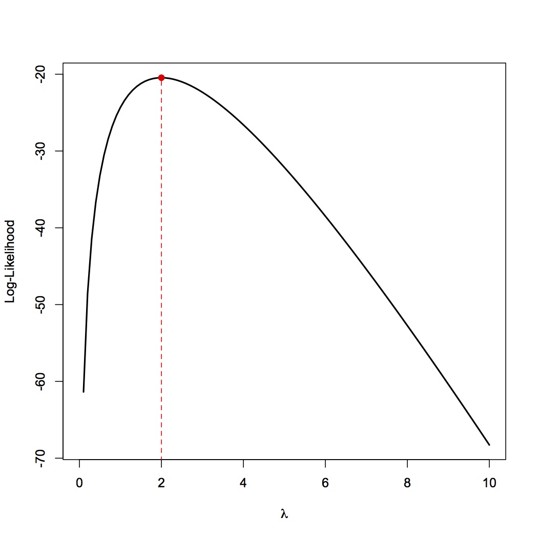
Suppose that we want to visualize the log-likelihood curve for data drawn from a Poisson distribution with an unknown parameter $\lambda$. The data we observe is {2,1,1,4,4,2,1,2,1,2}. In R, we can do this quite simply as:
my.data <- c(2,1,1,4,4,2,1,2,1,2)
pois.ll<- function(x) return(sum(dpois(my.data,lambda=x,log=TRUE)))
pois.ll <- Vectorize(pois.ll)
curve(pois.ll, from=0,to=10, lwd=2, xlab=expression(lambda),ylab="Log-Likelihood")
We already know (based on analytic solutions) that the MLE for $\lambda$ in a Poisson distribution is just the sample mean, which comes out to 2 in this case. Thus, we can mark it on the log-likelihood curve to produce the following graph:
If we wanted to maximize the log-likelihood in R (on the parameter space [0,100], chosen because it’s sufficiently wide to encompass the MLE), we could have done:
opt <- optimize(pois.ll, interval=c(0,100),maximum=TRUE)
opt$maximum # gives MLE
opt$objective # gives value of log-likelihood at MLE
R confirms our analytic solution.
Theory of Maximum Likelihood Estimation
Why do we use maximum likelihood estimation? It turns out that subject to regularity conditions the following properties hold for the MLE:
-
Consistency: as sample size ($n$) increases, the MLE ($\hat{\theta}_{MLE}$) converges to the true parameter, $\theta_0$. \(\hat{\theta}_{MLE} \overset{p}{\longrightarrow} \theta_0\)
-
Normality: As sample size ($n$) increases, the MLE is normally distributed with a mean equal to the true parameter ($\theta_0$) and the variance equal to the inverse of the expected sample Fisher information at the true parameter. However, using the consistency property of the MLE, we can use the inverse of the observed sample Fisher information evaluated at the MLE, denoted as $\mathcal{J}n(\hat{\theta}{MLE})$ to approximate the variance. The observed sample Fisher information is the negation of the second derivative of the log-likelihood curve. \(\hat{\theta}_{MLE} \sim \mathcal{N} \left(\theta_0, \Big(\underbrace{- \Big( \dfrac{\partial^2 \ell(\theta|\mathbf{x})}{\partial \theta^2} \Big|_{\theta=\hat{\theta}_{MLE}} \Big)}_{\mathcal{J}_n(\hat{\theta}_{MLE})} \Big)^{-1} \right)\)
-
Efficiency: maximum likelihood estimation generally provides the lowest variance as sample size increases.
